Announcing tidybayes + ggdist 3.0

Support for true gradients in R 4.1

We’ll use the following libraries for the demos below:

library(ggdist)
library(tidybayes)
library(ggplot2)
library(dplyr)
library(distributional)
library(modelr)
library(brms)

theme_set(theme_ggdist())

If you are using R >= 4.1, fills and alphas that vary within a slab in geom_slabinterval() can now be drawn as true gradients rather than segmented polygons by setting fill_type = "gradient". This substantially improves the appearance of gradient fills in graphics engines that support it:

dist_df = data.frame(
  group = c("a","b","c","d"),
  mean = 1:4,
  sd = c(1.6,1.4,1.2,1)
)

dist_df %>%
  ggplot(aes(x = group, dist = dist_normal(mean, sd), fill = group)) +
  stat_dist_gradientinterval(fill_type = "gradient") +
  scale_fill_brewer(palette = "Dark2") +
  ggtitle(
    'stat_dist_gradientinterval(fill_type = "gradient")',
    'aes(dist = dist_normal(mean, sd))'
  )

Because not all graphics engines support fill_type = "gradient", it is not turned on by default at the moment. You can omit fill_type = "gradient" and the gradients will still be displayed, but they make look “choppy”. For more on support for “true” gradients in R 4.1, see Paul Murrell’s blog post on the topic.

Improved support for discrete distributions

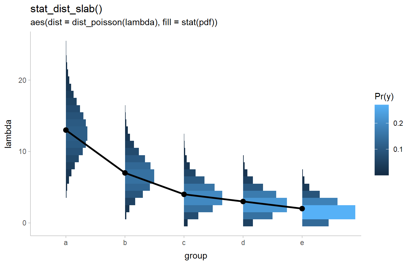
There are various improvements to support for discrete distributions, including better automatic binwidth selection for discrete distributions in geom_dotsinterval() and the automatic detection of discrete distributions in stat_dist_slabinterval(). The latter allows discrete analytical distributions to be automatically displayed as histograms:

tibble(
  group = c("a","b","c","d","e"),
  lambda = c(13,7,4,3,2)
) %>%
  ggplot(aes(x = group)) +
  stat_dist_slab(aes(dist = dist_poisson(lambda), fill = stat(pdf))) +
  geom_line(aes(y = lambda, group = NA), size = 1) +
  geom_point(aes(y = lambda), size = 2.5) +
  labs(fill = "Pr(y)") +
  ggtitle(
    "stat_dist_slab()", 
    "aes(dist = dist_poisson(lambda), fill = stat(pdf))"
  )

The improved support for discrete distributions in stat_dist_slabinterval() was precipitated by a discussion with Isabella Ghement.

Support for the new posterior package

Tidybayes and ggdist now support the posterior package, and in particular the new rvar datatype. All of the existing stat_dist... geoms in ggdist can be passed rvars using the dist aesthetic (just like with objects from distributional).

Tidybayes also now has a variety of functions suffixed with _rvars instead of _draws which work similarly to their _draws counterparts. To demo them, let’s use the palmerpenguins dataset. Here is the body mass of three penguin species broken down by sex:

data(penguins, package = "palmerpenguins")

penguins %>%
  na.omit() %>%
  ggplot(aes(y = species, x = body_mass_g, color = sex)) +
  stat_dots(position = "dodge", shape = 19, size = 0) +
  scale_color_brewer(palette = "Set2", guide = guide_legend(reverse = TRUE))

Males tend to be heavier than females. Let’s fit a simple model to predict sex based on body mass and species:

m_penguin = brm(
  # for this simple example I'm not using a varying slope, e.g. 
  # (body_mass_g|species), though that probably would be better
  sex ~ body_mass_g + (1|species), 
  data = penguins, 
  family = "bernoulli", 
  file = "tidybayes-ggdist-3-0-m2.rds"
)

The traditional way of pulling out parameters from a model in tidybayes has been to pull them out into a long-format data frame of draws. For example, we could use tidybayes::spread_draws() to pull draws from the global intercept and the species-specific random offsets as follows:

m_penguin %>%
  spread_draws(r_species[species,coef], Intercept)

## # A tibble: 12,000 x 7
## # Groups:   species, coef [3]
##    species coef      r_species .chain .iteration .draw Intercept
##    <chr>   <chr>         <dbl>  <int>      <int> <int>     <dbl>
##  1 Adelie  Intercept      2.43      1          1     1     0.882
##  2 Adelie  Intercept      2.57      1          2     2     1.05 
##  3 Adelie  Intercept      2.68      1          3     3     1.07 
##  4 Adelie  Intercept      3.10      1          4     4     1.34 
##  5 Adelie  Intercept      5.27      1          5     5    -0.678
##  6 Adelie  Intercept      4.43      1          6     6    -0.451
##  7 Adelie  Intercept      1.90      1          7     7     1.84 
##  8 Adelie  Intercept      4.93      1          8     8    -1.57 
##  9 Adelie  Intercept      6.06      1          9     9    -1.68 
## 10 Adelie  Intercept      5.68      1         10    10    -1.73 
## # ... with 11,990 more rows

This results in a 12,000-row data frame that is (1) very useful for summarizing and plotting but (2) a bit hard to read.

Using the new posterior::rvar datatype and the tidybayes::spread_rvars() function, we can instead pull out these coefficients into long-format data frames of rvars:

m_penguin %>% 
  spread_rvars(r_species[species,coef], Intercept)

## # A tibble: 3 x 4
##   species   coef        r_species Intercept
##   <chr>     <chr>          <rvar>    <rvar>
## 1 Adelie    Intercept   3.6 ± 2.0  0.22 ± 2
## 2 Chinstrap Intercept   3.3 ± 2.0  0.22 ± 2
## 3 Gentoo    Intercept  -6.4 ± 2.1  0.22 ± 2

The rvar datatype acts like a normal vector or array (including supporting many common functions and operators), but internally stores the full sample corresponding to each cell in the array. When printed, these draws are summarized to their mean and standard deviation. You can plot these objects using the stat_dist_... family in ggdist:

m_penguin %>% 
  spread_rvars(r_species[species,coef], b_Intercept) %>%
  mutate(species_intercept = b_Intercept + r_species) %>%
  ggplot(aes(y = species, dist = species_intercept)) +
  stat_dist_halfeye() +
  xlab("Species-specific intercept")

This intercept isn’t very interpretable, so let’s instead use it with the slope (the coefficient on body_mass_g) to calculate the body mass for each species where we’d expect a 50-50 chance of an individual being male or female. This is just based on a re-arrangement of the equation for the log-odds of being male:

\[ \begin{align*} \textrm{logit}(\Pr(\textrm{male})=0.5) &= \beta_\textrm{body_mass}\textrm{body_mass}+\beta_\textrm{intercept}\\ \implies \textrm{body_mass} &= \frac{-\beta_\textrm{intercept}}{\beta_\textrm{body_mass}} & \textit{because }\textrm{logit}(0.5)=0 \end{align*} \]

We can overlay this crossing-point on the orginal dotplot. We’ll also use the fact that side can now vary as an aesthetic to plot the dotplots flipped for male versus female penguins (described in more detail in the next section):

m_penguin %>% 
  spread_rvars(r_species[species,coef], b_Intercept, b_body_mass_g) %>%
  mutate(species_intercept = b_Intercept + r_species) %>%
  mutate(species_50pct = -(species_intercept)/b_body_mass_g) %>%
  ggplot(aes(y = species)) +
  stat_dots(
    aes(
      x = body_mass_g, color = sex, 
      side = ifelse(sex == "male", "top", "bottom")
    ),
    shape = 19, size = 0, data = na.omit(penguins), scale = 0.5
  ) +
  stat_dist_pointinterval(aes(dist = species_50pct)) +
  scale_color_brewer(palette = "Set2", guide = guide_legend(reverse = TRUE))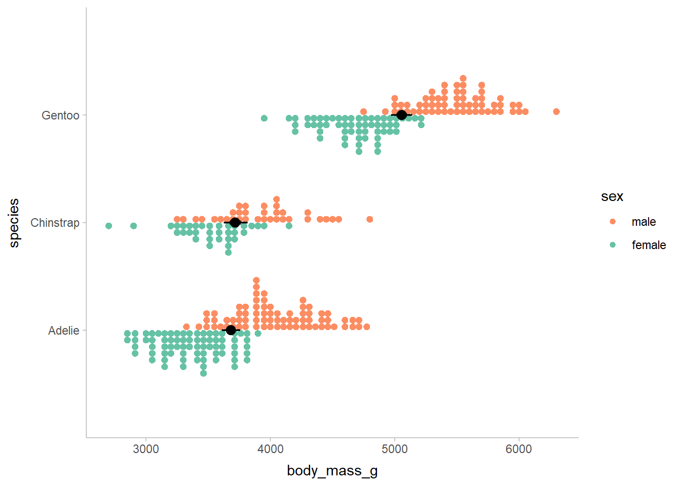

We can also use modelr::data_grid() to made a grid of predictors and then use add_epred_rvars() to add random variables representing draws from the expectation of the posterior predictive distribution to it. This is similar to how add_fitted_draws() (now renamed to add_epred_draws(), see note below) works in the classic tidybayes workflow, but instead of returning long data frames of draws, it uses the rvar datatype to encapsulate the draws for each row of the prediction grid. This makes the output much easier to read (I’ll also show an example of visualizing this in the next section):

penguins %>%
  data_grid(
    species, 
    body_mass_g = seq_range(body_mass_g, n = 50)
  ) %>%
  add_epred_rvars(m_penguin, value = "Pr(sex = male)")

## # A tibble: 150 x 3
##    species body_mass_g  `Pr(sex = male)`
##    <fct>         <dbl>            <rvar>
##  1 Adelie        2700   0.0011 ± 0.00098
##  2 Adelie        2773.  0.0018 ± 0.00148
##  3 Adelie        2847.  0.0029 ± 0.00222
##  4 Adelie        2920.  0.0048 ± 0.00332
##  5 Adelie        2994.  0.0079 ± 0.00495
##  6 Adelie        3067.  0.0131 ± 0.00733
##  7 Adelie        3141.  0.0215 ± 0.01076
##  8 Adelie        3214.  0.0353 ± 0.01558
##  9 Adelie        3288.  0.0575 ± 0.02212
## 10 Adelie        3361.  0.0926 ± 0.03054
## # ... with 140 more rows

You can also convert to/from the data-frame-of-rvars format and the long-data-frame-of-draws format using nest_rvars() and unnest_rvars(). See the tidy-posterior vignette for more on extracting and visualizing rvars with tidybayes.

Some of the core tidying functionality in tidybayes has also been rebuilt on top of posterior, which means tidybayes should support even more model types and benefit from efficiency improvements in posterior. This means that cmdstanr is now supported, for example.

Side, justification, and scale are now aesthetics

For geom_slabinterval(), side, justification, and scale can now be used as aesthetics instead of parameters, allowing them to vary across slabs within the same geom.

These changes make it possible to do things like recreate Ladislas Nalborczyk’s logit dotplot without having to manually figure out dotplot binwidths; here we restrict both dotplots to less than 1/3 of the available space with scale = 1/3 and geom_dots() does the hard work of figuring out how big the dots should be to achieve that:

penguins %>%
  filter(species == "Gentoo") %>%
  data_grid(
    species = "Gentoo",
    body_mass_g = seq_range(body_mass_g, n = 50, expand = 0.1)
  ) %>%
  add_epred_rvars(m_penguin, value = "Pr(sex = male)") %>%
  ggplot(aes(x = body_mass_g)) +
  stat_dots(
    aes(
      y = as.numeric(sex == "male"), 
      side = ifelse(sex == "male", "bottom", "top")
    ), 
    data = filter(penguins, species == "Gentoo"),
    na.rm = TRUE, scale = 1/3
  ) +
  stat_dist_lineribbon(
    aes(dist = `Pr(sex = male)`), 
    alpha = 1/4, fill = "#08306b"
  ) +
  coord_cartesian(expand = FALSE) +
  scale_fill_brewer() +
  labs(
    title = "stat_dots(scale = 1/3)",
    subtitle = 'aes(side = ifelse(sex == "male", "bottom", "top"))',
    x = "Body mass (g) of Gentoo penguins",
    y = "Pr(sex = male)"
  )

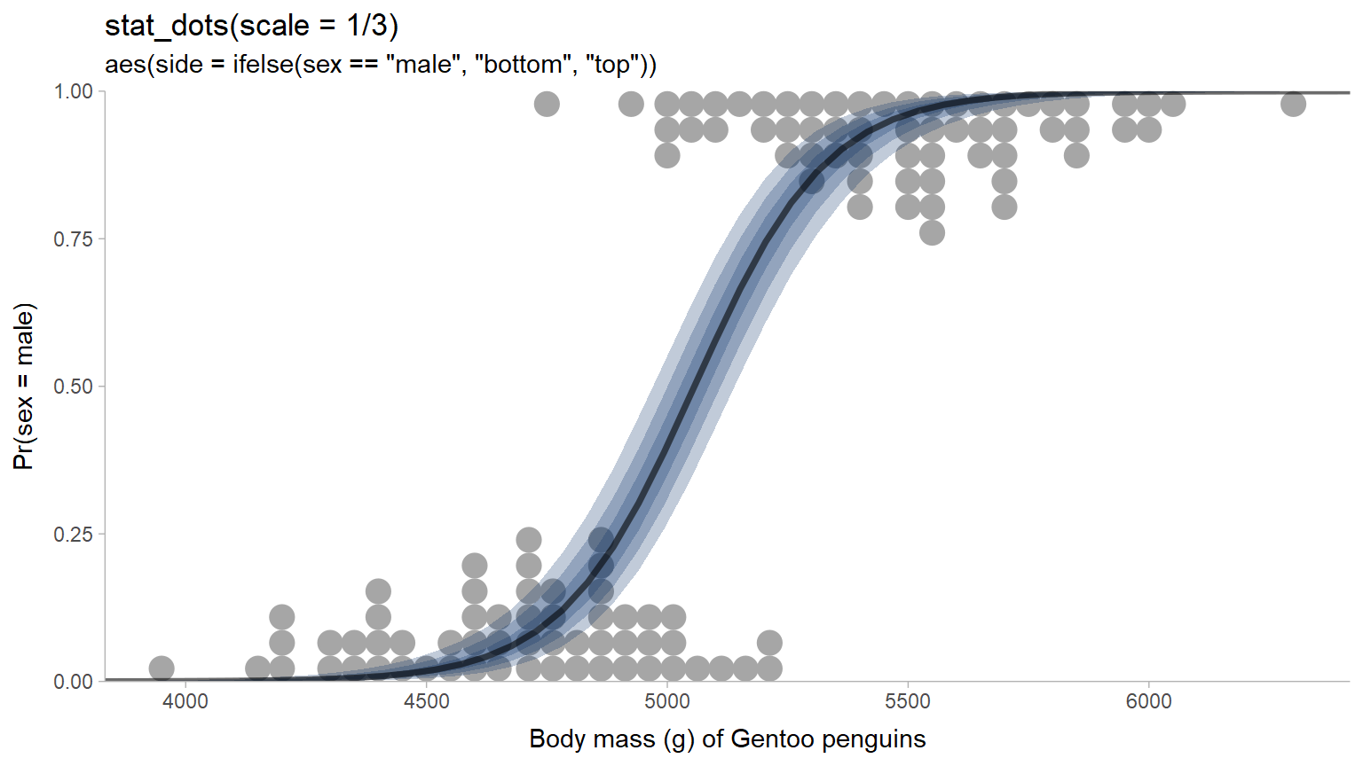
This example also shows the use of rvars with stat_dist_lineribbon().

Making scale, side, and justification into aesthetics was precipitated by a discussion with Dominique Makowski and Brenton Wiernik in their attempts to recreate the logit dotplot for the see package.

Re-organization of tidybayes prediction functions

The [add_]XXX_draws() functions (predicted_draws(), add_predicted_draws(), etc) have been substantially restructured:

• add_fitted_draws() and fitted_draws() are now deprecated, along with their scale = c("response", "linear") argument. Several years’ teaching experience has demonstrated that “fitted” is a very confusing name for students. Use the more-specific [add_]linpred_draws() if you want draws from the linear predictor or the new [add_]epred_draws() if you want draws from the expectation of the posterior predictive (which is what fitted_draws() was most typically used for).
• Arguments for renaming output columns are now all called value, but retain function-specific default column names. E.g. the prediction argument for predicted_draws() is now spelled value but has a default of ".prediction". One breaking change is that the default output column for linpred_draws() is now ".linpred" instead of ".value". This should make it easier to combine outputs across multiple functions while also making it easier to remember the name of the argument that changes the output column name.
• The n argument is now spelled ndraws* to be more consistent with terminology in the posterior package and to prevent partial argument name matching bugs with newdata.
• The first argument to all of these functions is now object instead of model, in order to match with argument names in posterior_predict(), etc. This was necessary to prevent partial argument name matching bugs with certain model types in rstanarm that have an m argument to their prediction functions.

See the function documentation or examples from the vignettes for more.

Along with this restructuring, the epred_draws(), linpred_draws(), and predicted_draws() functions should now support any models that implement posterior_epred(), posterior_linpred(), and posterior_predict() so long as they take a newdata argument.

New dodging behavior for geom_slabinterval

The positioning of geom_slabinterval() family geoms is now a bit different, which should make it easier to line up intervals with other geoms when using position_dodge(). Here’s an example of using position = "dodge" with ggdist::stat_dist_halfeye(), ggplot2::geom_rect(), and ggplot2::geom_point():

dist_df %>%
  ggplot(aes(
    x = "a", dist = dist_normal(mean, sd), fill = group, color = group
  )) +
  stat_dist_halfeye(position = "dodge", color = "black") +
  geom_rect(
    aes(xmin = 1, xmax = 2, ymin = -3, ymax = 7),
    position = "dodge",
    alpha = 0.1
  ) +
  geom_point(
    aes(y = 0),
    position = position_dodge(width = 1),
    shape = 1, size = 4, stroke = 1.5
  ) +
  scale_fill_brewer(palette = "Set2") +
  scale_color_brewer(palette = "Dark2")

Notice how the points from geom_point() line up with the horizontal positions of the intervals: in previous versions of ggdist this would not work. However, the slabs do not perfectly line up with the dodged bounding boxes shown with geom_rect(). This is because ggplot2::position_dodge() does not preserve the relative positions of points and bounding boxes when dodging. This can cause slabs to get close to (or in extreme cases, be drawn slightly outside) plot bounds.

If you encounter this problem, the new ggdist::position_dodgejust(), a “justification-preserving dodge”, can be used:

dist_df %>%
  ggplot(aes(
    x = "a", dist = dist_normal(mean, sd), fill = group, color = group
  )) +
  stat_dist_halfeye(position = "dodgejust", color = "black") +
  geom_rect(
    aes(xmin = 1, xmax = 2, ymin = -3, ymax = 7),
    position = "dodge",
    alpha = 0.1
  ) +
  geom_point(
    aes(y = 0),
    # use position_dodgejust here to match the justification
    # of the point to the halfeye when dodging
    position = position_dodgejust(width = 1, justification = 0),
    shape = 1, size = 4, stroke = 1.5
  ) +
  scale_fill_brewer(palette = "Set2") +
  scale_color_brewer(palette = "Dark2")

These changes to dodging were precipitated by some feedback from Brenton Wiernik.

Improvements for package developers

Two big changes in ggdist are aimed at making it easier for other package developers to build on it:

• The automatic bin selection algorithm and and binning algorithm used by geom_dotsinterval() have been factored out and exported as ggdist::find_dotplot_binwidth() and ggdist::bin_dots().

• Dependencies have been substantially reduced in both ggdist and tidybayes. Particularly in ggdist the hope is that the geoms will now be more suitable for use by other package developers that want to maintain smaller dependency trees (thanks to Brenton Wiernik for the help).

Other new features and changes

Other new features include:

• Substantial improvements to the documentation of aesthetics and computed variables in geom_slabinterval(), stat_slabinterval(), and company, listing all custom aesthetics, computed variables, and their usage. See the aesthetics documentation or the computed variables documentation.

• Previously, curve_interval() used a common (but naive) approach to finding a cutoff on data depth to identify the X% “deepest” curves, simply taking the envelope around the X% quantile of curves ranked by depth. This is quite conservative and tends to create intervals that are too wide; curve_interval() now searches for a cutoff in data depth such that X% of curves are contained within its envelope (#67).

For more information on other minor changes, see the ggdist changelog or the tidybayes changelog.